Formal Methods for PDEs

Partial differential equations (PDEs) model nearly all of the physical systems and processes of interest to scientists and engineers. Some well-known examples include the Navier-Stokes equation for fluid mechanics, the Maxwell equations for electromagnetics, the Schrödinger equation for quantum mechanics, the heat equation and the wave equation. The analysis of these and other PDEs has had a tremendous impact on society by enabling our understanding of thermal, electrical, fluidic and mechanical processes.

While a mature field, the study of PDEs is often approached through simulations in which approximate models obtained through spatio-temporal discretization techniques, such as the Finite Element Method (FEM), are solved numerically. These methods, however, do not allow for rigorous guarantees that a system satisfies a complex specification. Other approaches generalizing classic Ordinary Differential Equations (ODEs) tools such as Lyapunov analysis and backstepping do provide some guarantees and can be used to obtain boundary control strategies for a wide variety of PDEs. However, they are restricted to classical control objectives such as stabilization and cost optimization.

The formal statement of specifications and the development of analysis techniques that can guarantee their satisfaction by design has been the main focus of the formal methods field. During the past decades, many specification languages have been defined, such as Linear Temporal Logic (LTL) and Signal Temporal Logic (STL). Originally, these logics have been applied to the study of finite systems, although more recently abstraction procedures have been developed to reduce problems with ODEs to finite models (for example through state space discretization or mixed-integer linear program (MILP) encodings). However, these techniques cannot be immediately applied to the analysis of PDEs due to the lack of spatial information in the formal language. This issue was first addressed in in the context of spatially distributed systems, which can be viewed as PDEs in a discretized spatial domain. In their work, the authors view the system state as an image and define a formal language with explicit spatial information called Linear Superposition Logic (LSSL) based on quadtrees, a tree-based abstraction of the system. A variant of LSSL with quantitative semantics, Tree Spatial Superposition Logic (TSSL), was used for (steady-state) pattern synthesis in reaction diffusion systems, and a formal language combining TSSL and STL, Spatial Temporal Logic (SpaTeL), allows the synthesis of dynamical patterns. The specification of patterns in these logics is difficult, however, and machine learning techniques are needed in order to obtain logic formulas corresponding to a set of examples of the desired pattern, which is not always available or desirable for some applications where the system behavior must be specified a priori. More recently, a new spatio-temporal logic called STREL was introduced in to specify the behavior of mobile and spatially distributed Cyber-Physical Systems.

One of the major drawbacks of these methods is the issue of scalability. Both of the main approaches, automata and optimization, quickly become unfeasible when the system dimension increases, which poses a problem when dealing with infinite-dimensional systems such as PDEs. In the case of optimization based techniques, a recent trend has focused on decentralized synthesis and verification where the coupling between subsystems is formally captured in Assume-Guarantee Contracts (AGCs). However, the key assumption of monotonicity is not present in PDE systems.

Besides classical problems that focus on the temporal evolution of the state of the system, PDEs allow for a different kind of problems where the aim is to specify the intrinsic behavior of the system through its so called constitutive response. In this case, instead of designing boundary control inputs, the engineer is tasked with the design of the geometry of a structure that exhibits the desired mechanical or thermal properties. The traditional approach to this problem, topology optimization is not enough to tackle both geometric and material nonlinearity.

Boundary Control

In order to solve the classical boundary control problems through the use of formal methods, we’ve developed a formal language called Spatial-STL (S-STL) and a framework that reformulates a verification or control synthesis problem for a PDE system into an optimization problem for a system of difference equations that can be encoded and solved as a Mixed-Integer Linear Program (MILP). As an example of the kind of properties we can describe with S-STL, consider the following:

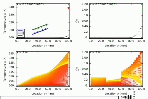
Consider a metallic rod of 100mm. The temperature at one end of the rod is fixed at 300 kelvin, while a heat source is applied to the other end. The temperature of the rod follows a linear 1D heat equation. We want the temperature distribution of the rod to be within 3 kelvin of the linear profile $\mu(x) = \frac{x}{4} + 300$ at all times between 4 and 5 seconds in the section between 30 and 60 mm. Furthermore, the temperature should never exceed 345 kelvin at the point where the heat source is applied ($x=100$). We can formulate such a specification using the following S-STL formula:

\begin{equation}\label{eq:phi_ex} \begin{aligned} \phi_{ex} = &\mathbf{G}_{[4,5]} \big((\forall x \in [30,60] : u(x) - (\frac{x}{4} + 303) < 0 ) \land \\
&\quad (\forall x \in [30, 60] : u(x) - (\frac{x}{4} + 297) > 0)\big) \land \\
&\mathbf{G}_{[0, 5]} (\forall x \in [100, 100] : u(x) - 345 < 0) \end{aligned} \end{equation}

Note that S-STL admits quantitative semantics similar to STL (see the templogic project page for a quick introduction.)

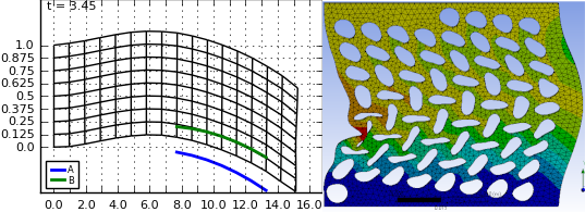
We implemented this framework in a Python tool called FEMFormal. In FEMFormal, you can define boundary control problems in 1D and 2D linear heat and wave equations, as well as some non-linear 1D wave equations. Then, you can solve verification and synthesis problems with S-STL specifications such as the one above. For example, for a mixed steel and brass rod, our tool obtains the following solution:

You can see more solved examples as well as how to use FEMFormal here.

Constitutive Response Design

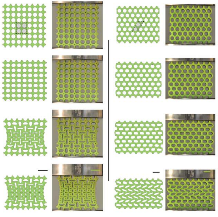
Suppose we now want to produce a wide variety of mechanical behaviors out of a single material. For example, can we give an elastic material a tunable, effective yield point, or make it strain harden or soften at a specified amount of displacement? This response to loading can be determined from the stress-strain curve, which serves as a fundamental piece of information that describes the global mechanical properties of structures and materials. Recent advances in mechanical metamaterials have shown that it is possible to tailor the relationship between stress and strain of a particular material through structural patterning.

In order to formally specify the desired response of the structure, we developed a formal language over stress-strain curves and adapted S-STL for this purpose. Then, we proposed an optimization procedure based on gradient-free optimization algorithms and simulation.

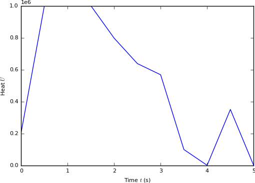
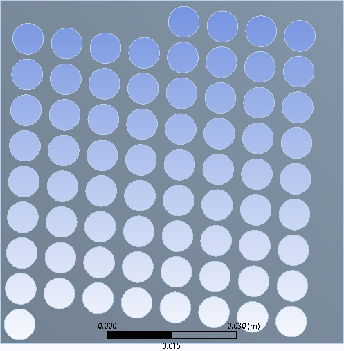
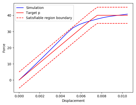
Consider the following example of this process: a square sheet of rubber of side $L = 8cm$ and thickness $h = 1cm$ is drilled with circular holes of radius $r$ constrained to be within the interval $[0.3cm, 0.4cm]$ and distributed in a lattice given by the vectors $v_1, v_2 \in \mathbb{R}^2$ such that they do not intersect. The constitutive response was obtained as a positive force-displacement curve by loading the material with a force $F(t)$ applied uniformly across the top surface such that the discplacement at the top surface increases linearly from 0 to 1.05cm in 3.5 seconds. The specification in this case is to have the force-displacement curve of the material to be within $\epsilon$ tolerance of a target curve $p$, which can be expressed in S-STL as the following formula:

\begin{equation} \begin{aligned} \phi = \forall x \in {(0, L)} : \mathbf{G}_{[0, T]} (F < p(d_2(x)) + \epsilon \land F > p(d_2(x)) - \epsilon) \\
p(d) = \begin{cases} \frac{40}{7.5 \cdot 10^{-3}} d & d < 7.5 \cdot 10^{-3} \\
40 & d > 7.5 \cdot 10^{-3} \end{cases} \end{aligned} \end{equation}

where $d_2(x)$ represents the displacement of the top boundary at $x$, $F$ is the applied force, the temporal operator $\mathbf{G}_{[0, T]} \psi$ means that $\psi$ must be satisfied at all times in the interval and the spatial operator $\forall x \in {(0, L)} : \psi$ means that $\psi$ must be satisfied at all points in the interval.

We solved this problem using differential evolution to find the best pattern with respect to the S-STL score of the specification $\phi$. We generate simulations of the system using the Finite Element Method simulator ANSYS. After 280 evaluations performed in about 38 hours, we obtained the following pattern:

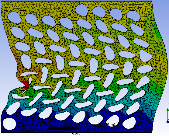
This pattern results in a S-STL score of 0.641, with the following force-displacement curve (compared to the target curve and its tolerance):