Temporal Logics Library

Temporal logics are formal languages capable of expressing properties of system (time-varying) trajectories. Besides the usual boolean operators, temporal logics introduce temporal operators that capture notions of safety (“the system should always operate outside the danger zone”), reachability (“the system is eventually able to enter a desired state”), liveness (“the system always eventually reaches desired states”), and others. Once a property is expressed, automatic tools based on automata theory, optimization or probability theory are able to check wether a system satisfies the property, or synthesize a controller such that the system is guaranteed to satisfy the specification.

I have organized most of the Python code implementing a few of the temporal logics used in my thesis in the library Templogic. In particular, I have included several logics that admit quantitative semantics (see below), along with functionality that pertains to the logic itself, such as parsing, inference and mixed-integer encodings.

Quantitative Semantics

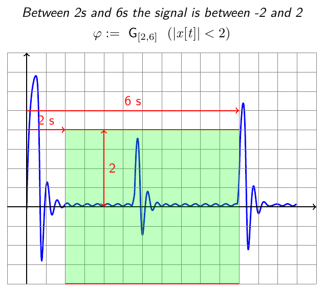
For some scenarios, a binary measure of satisfaction is not enough. For example, one might want to operate a system such that safety is not only guaranteed but robustly guaranteed. In other applications, a not satisfying best effort might provide an engineer with clues about mistakes in the specification or guide more expensive algorithms towards satisfaction. For these situations, some temporal logics can be equiped with quantitative semantics, i.e., a real score $r$ such that a trajectory satisfies a specification if and only if $r > 0$. If one considers a temporal logic formula as the subset of trajectories that satisfy it, the score $r$ can be interpreted as the distance of a trajectory to the boundary of this set.

Consider for example Signal Temporal Logic (STL), a temporal logic based on Lineal Temporal Logic (LTL) that defines temporal bounds for its temporal operators and uses inequalities over functions of the system state as predicates. For example in STL one can express the property “always between 0 and 100 seconds the $x$ component of the system state cannot exceed the value 50, and eventually between 0 and 50 seconds the $x$ component of the system must reach a value between 5 and 10 and stay within those bounds at all times for 10 seconds”, which would be written as the formula:

$$ \phi = G_{[0, 100]} x < 50 \wedge F_{[0, 50]} (G_{[0, 10]} (\lnot (x < 5) \wedge x < 10)) $$

You can define $\phi$ using Templogic as follows:

from templogic.stlmilp import stl 

# `labels` tells the model how each state component at time `t` is represented
# It can also be a function of t that returns the list of variables at time `t`
labels = [lambda t: t]

# Predicates are defined as signal > 0
signal1 = stl.Signal(labels, lambda x: 50 - x[0])
signal2 = stl.Signal(labels, lambda x: 5 - x[0])
signal3 = stl.Signal(labels, lambda x: 10 - x[0])

f = stl.STLAnd(
      stl.STLAlways(bounds=(0, 100), arg=stl.STLPred(signal1))
      stl.STLEventually(
        bounds=(0, 50),
        arg=stl.STLAlways(
          bounds=(0, 10),
          arg=stl.STLAnd(
            args=[
              stl.STLNot(stl.STLPred(signal2)),
              stl.STLPred(signal3)
            ]))))

The score or robustness of a trajectory $x(t)$ with respect to the specification $\phi$ can be defined as follows:

$$ \begin{multline} r(x(t), \phi) = \min \{\min_{t \in [0, 100]} 50 - x(t), \\
\max_{t \in [0, 50]} (\min_{t \in [0, 10]} (\min \{-(5 - x(t)), 10 - x(t)\})) \} \end{multline} $$

In Templogic, you must define a model that understands how to translate state variables at time t used in signals:

class Model(stl.STLModel):
  def __init__(self, s) -> None:
    self.s = s
    # Time interval for the time discretization of the model
    self.tinter = 1

  def getVarByName(self, j):
    # Here `j` is an object that identifies a state variable at time `t` 
    # in the model, generated by the functions in `labels` above. 
    # In our case it is simply the index in the array that contains the 
    # trajectory
    return self.s[j]

You can then compute the score for a particular model:

s = [0, 1, 2, 4, 8, 4, 2, 1, 0, 1, 2, 6, 2, 1, 5, 7, 8, 1]
model = Model(s)
score = stl.robustness(f, model)

Mixed-Integer Linear Programming

An obvious framework to work with temporal logics with quantitative semantics would be to reformulate verification and synthesis problems as optimization problems, where the objective is to maximize the score $r$. However, as can be seen above, the definition of the score is non-convex and discontinuous, which makes it particularly difficult to include directly either as an objective function or as a constraint in efficient optimization algorithms, such as those used in Linear Programming. Instead, an equivalent reformulation can be used to transform the score definition into a series of mixed-integer linear constraints. The solution of Mixed-Integer Linear Programs (MILPs) is in general very expensive (double exponential), but very good heuristic techniques can be used to efficiently solve interesting problems in practice. As an example, consider the following MILP reformulation of the function $\min \{x, y\}$:

$$ \begin{aligned} r \leq x \\
r \leq y \\
r > x - Md \\
r > y - Md \\
d \in \{0, 1\} \end{aligned} $$

where $M$ is a sufficiently big number chosen a priori. The auxiliary variable $r$ can now be used as optimization objective or as a constraint (for example $r > 0$ for satisfaction). As seen above, robustness in STL are defined as nested $\max$ and $\min$ operations and can be fully encoded in this fashion. In Templogic, we define encodings for the popular MILP solver Gurobi. You can create an MILP model and add the robustness of the STL formula f defined above as follows:

from templogic.stlmilp import stl_milp_encode as milp

m = milp.create_milp("test")

# Define here your model. Make sure you label each variable representing
# a system variable at time `t` consistently with the `labels` parameter
# to the STL Signals. For example labels may be defined as:
# labels = [lambda t: f"X_0_{t}"]
# which would, for t=5, fetch the variable `X_0_5` from the Gurobi model
m.addVar(...)
m.addConstr(...)

# `r` contains a Gurobi variable with the robustness of f.
r, _ = milp.add_stl_constr(m, "robustness", f)

# You can use this variable in constraints
m.addConstr(r > 0)

# or set a weight in the objective function for it
r.setAttr("obj", weight)

You can find more helper functions in the stl_milp_encode module.

STL Inference

STL inference is the problem of constructing an STL formula that represents “valid” or “interesting” behavior from samples of “valid” and “invalid” behavior. This is often called the two-class classification problem in machine learning. We developed a decision-tree based framework for solving the two-class classification problem involving signals using STL formulae as data classifiers. We refer to it as framework because we didn’t just proposing a single algorithm but a class of algorithms. Every algorithm produces a binary decision tree which can be translated to an STL formula and used for classification purposes. Each node of a tree is associated with a simple formula, chosen from a finite set of primitives. Nodes are created by finding the best primitive, along with its optimal parameters, within a greedy growing procedure. The optimality at each step is assessed using impurity measures, which capture how well a primitive splits the signals in the training data. The impurity measures described in this paper are modified versions of the usual impurity measures to handle signals, and were obtained by exploiting the robustness score of STL formulas.

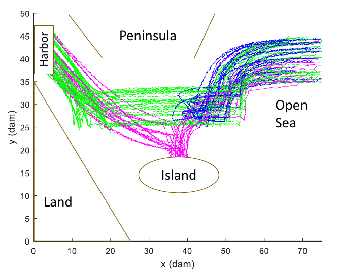
Our STL inference framework is implemented in the templogic.stlmilp.inference package, and a command line interface is provided. As an example, consider the following naval surveillance scenario: assume you have a set of trajectories of boats approaching a harbor. A subset of trajectories corresponding with normal behavior are labeled as “valid”, while the others, corresponding with behavior consistent with smuggling or terrorist activity, are labeled “invalid”.

You can encode this data in a Matlab file with three matrices:

• A data matrix with the trajectories (with shape: number of trajectories x dimensions x number of samples),
• a t column vector representing the sampling times, and
• a labels column vector with the labels (in minus-one-plus-one encoding).

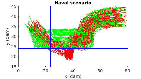
You can find the .mat file for this example in templogic/stlmilp/inference/data/Naval/naval_preproc_data_online.mat. In order to obtain an STL formula that represents “valid” behavior, you can run the command:

$ lltinf learn templogic/stlmilp/inference/data/Naval/naval_preproc_data_online.mat
Classifier:
(((F_[74.35, 200.76] G_[0.00, 19.84] (x_1 > 33.60)) & (((G_[237.43, 245.13] ...